Enter the Monetary Wonderland

Part 2:
Cycle of Paradox

Published: 30 August, 2018
Last Edited: 16 September, 2018
by Michio Suginoo

---

INTRODUCTION

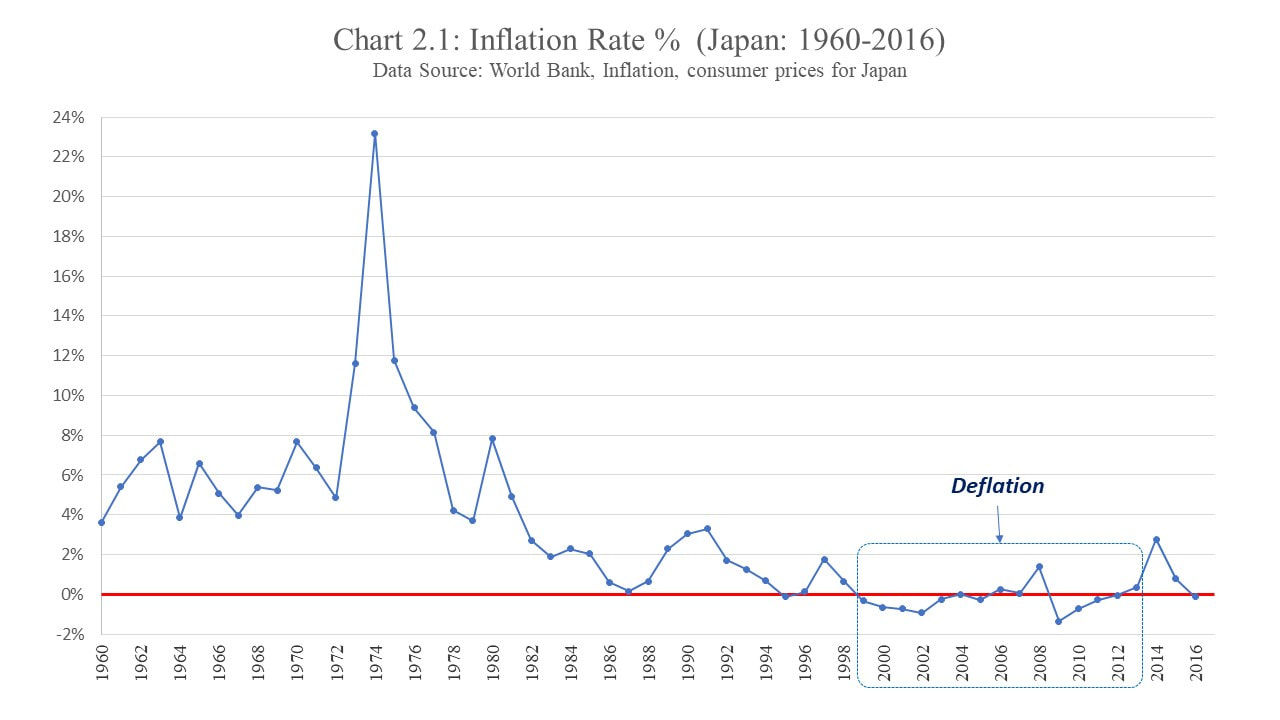
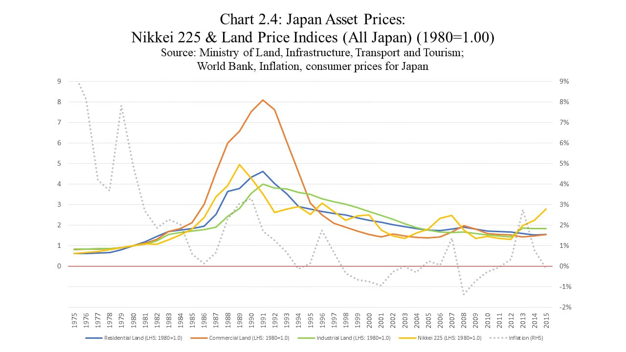
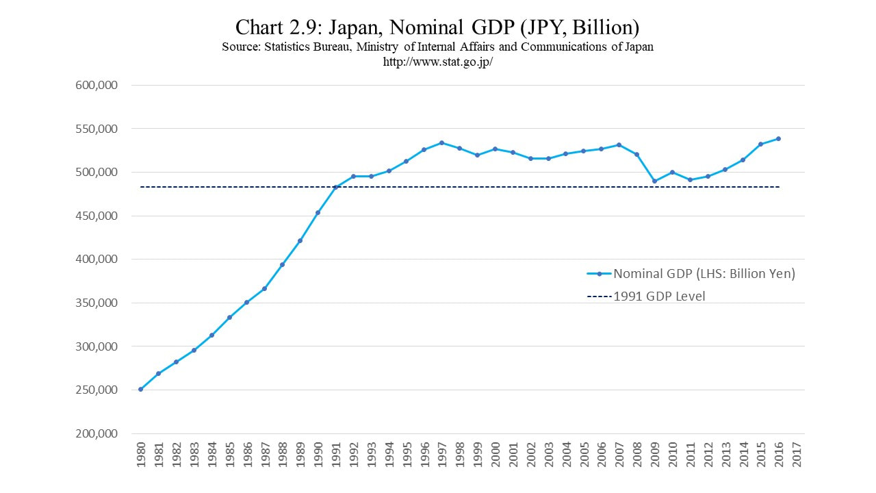
Part 1 of this reading compared two contrasting monetary wonderlands—deflationary Japan and inflationary Argentina—and illustrated how monetary conditions can shape our social, political, and economic behaviours. It also illuminated the interactive characteristic of the architecture of monetary wonderland: while a given set of monetary conditions shapes our particular collective behaviours, our monetary reality can also be shaped by our collective behaviours. In a way, our monetary reality, call it ‘Monetary Wonderland,' is a manifestation of a series of ‘feed-in and feed-back’ interactive dynamics between our collective behaviours and monetary reality.

Part 1 also hinted a cyclical nature of ‘Monetary Wonderland.’ Every time a new economic imbalance emerged, it was a consequence of earlier developments that had arisen from another old economic imbalance. As an example, Japan’s ‘Lost Decades’ was a product of the preceding debt-driven asset bubble during the second half of the 80s. The collapse of the asset bubble ruptured the bubble time psychology as well as the bubble time economic reality. As a result, the post-bubble economic reality transformed into a protracted deflationary stagnation, called ‘Lost Decades.’ Furthermore, as presented later, the asset bubble itself was also an unintended consequence of its preceding events. In a way, our ‘Monetary Wonderland’ is a temporal manifestation of chain reactions in its past. In this passage, our monetary reality did not gravitate toward an equilibrium, but rather ran from one disequilibrium to another.

With this cyclical notion in our mind, Part 2 goes a little deeper into the underlying mechanism of the cycle by examining how the cyclical nature manifested itself along Japan’s monetary experience since the 70s.

Shirakawa’s Paradoxical Cycle of Monetary Policy:

Masaaki Shirakawa, an ex-governor of the Bank of Japan from April 2008 to March 2013, expressed his insight of a paradox embedded in the conduct of monetary policy. Shirakawa illuminated how the success of monetary policy that had been aimed at economic stability paradoxically gave rise to unintended extreme economic imbalances and swung monetary reality from one extreme to another. Furthermore, he predicted that the conduct of conventional monetary policy could ultimately end up shaping an economic environment in which it becomes no longer effective. In Shirakawa’s perspective, the victory of monetary policy could defeat itself in the long run.

Now, I would like to integrate some other prominent economists’ insights into Shirakawa’s framework to illustrate the cyclical aspect of ‘Monetary Wonderland.’

The historical backdrop of the bubble formation:

To capture ‘Shirakawa’s Monetary Policy Paradox’, we examine Japan’s monetary experience starting with a victory of monetary policy over CPI inflation, which took place in a highly uncertain inflation period during the 70s.

In 1973, the first oil crisis caused a supply disruption in the global energy sector. Oil price surged from USD 3 per barrel to USD 10 per barrel within a year (Chart 2.3).  The rise in oil price transmitted inflationary pressure across the global economy. Japan was not an exception, registering 11.63% of annual average inflation rate in 1973 and 23% in 1974 (Chart 2.1). In an immediate response, the central bank made a decisive move to raise its policy rates to 9% in 1973 (Chart 2.2). As a result, CPI inflation gradually came down to 3.7% by 1979 (Chart 2.1), despite the fact that oil price continued rising up to USD 15 by 1979. As they made their success in containing inflation, BoJ lowered the policy rates gradually to the level of 3.5% by 1978.

The crisis in 1973 tested the central bank’s willingness and ability to restore both price and economic stabilities. And the victory of monetary policy embodied the central bank’s commitment and capability on price stability and shaped a firm public confidence on both price and economic stabilities.
 
The second oil crisis broke out in the context of the Iranian Revolution in 1979. The oil price TRIPLED to USD 45 per barrel from USD 15 per barrel (Chart 2.3). Nevertheless, the actual scale of the supply disruption was limited. As a result, the annual average inflation rate rose only up to 8% (Chart 2.1). The decisive monetary policy raised the policy rate up to 9% by 1980 and successfully contained the situation (Chart 2.2).

The formation of Japan’s Bubble during the 80s.

An interesting development was brewing in the asset prices at the turn of the 80s (Chart 2.4). As the market confirmed the decisive monetary policy at 9% in 1980, the asset prices started taking off (Chart 2.4) without waiting for a substantial drop in the policy rate (Chart 2.2). Between 1980 and 1984, during only four years, the commercial land price index (1980=1.0, all Japan average) already had DOUBLED; the residential land price index and the industrial land price index both (1980=1.0, all Japan average) had nearly DOUBLED; the price of the stock index, Nikkei 225, had MULTILIED by the factor of 1.5 times.

How can we explain such a rapid increase in these asset prices?

According to Shirakawa, the immediate increase in asset prices after the second oil crisis was a reflection of the solid public confidence in monetary policy in restoring economic stability. If the first oil shock was for the public to test the central bank’s ability to stabilise both prices and economy, the second oil shock was for them to act on it. Shirakawa emphasises the transformation in the psychology of market participants in response to the success of monetary policy:

“The success in attaining price stability lent support to public confidence in the central bank’s conduct of monetary policy. As a result, inflation expectations of private-sector economic entities became well anchored to a low-target inflation rate. Thus, imbalances in the economy began to appear in forms other than inflation of goods and services. Imbalances materialized in different forms such as increases in asset prices and growth of credit extension.” (Shirakawa, April 22, 2010, pp. 488-489)

As the inflation came down to 2% by 1985, the central bank lowered interest rates down to 5% (Chart 2.2). Now, a lower interest rate further justified the public expectation for sustainable stability in prices and economy. With a prospect in both a cheaper financing cost and a sustainable economic stability, the corporate sector increased debts to extend their investments, especially in commercial properties. The asset prices, reflecting the debt-driven over-investment, accelerated the surge in their price index (Chart 2.4).

Now, leaving Japan’s context for a while, in a general context, the public confidence on the monetary condition would penetrate into their prospect on the economy, and ultimately increase private demands. At an early stage, the supply side might catch up with the pace of the demand increase rather smoothly with their available underutilised supply capacity. As the demand rise continues, it transforms the psychology of the suppliers. Once an expectation emerges that the increasing demand would use up its existing supply capacity sooner or later, the expectation transmits into the prices. Then, a higher price would send a signal to the suppliers that it is the time to start building up additional capacity to catch up with the seemingly ever-rising hungry demand. It triggers a new trend of time consuming capital expenditure projects—constructions of new factories, commercial properties, and residential properties. Now, the supply side takes out finance and increases the demand for capital investment. This shapes an interesting loop: an increase in demand leads to a supply expansion, which feeds back into the finance-fed demand (for capital investment). Supply capacity expansion is a time-consuming capital investment process. A substantial time lag between the pace of the rising demand and that of the ‘supply catch-up’ would cause a temporary supply shortage. This temporary economic imbalance sends the market prices higher and higher. Now let’s go back to Japan’s story.

Between 1980 and 1986, the commercial land price index TRIPLED; the residential land price index more than DOUBLED; the industrial land price index little less than DOUBLED; the price of Nikkei 225 nearly TRIPLED (Chart 2.4). During the same period, despite an acute surge in the asset prices, the inflation rate of prices of goods and services (call it ‘consumer price inflation’ going-forward) continued declining to 0.14%. This divergence in price behaviours between assets and the consumer prices (goods and services) served as a source of brewing the very problem, debt-driven asset bubble. With an intense focus on the consumer price inflation behaviour, the central bank maintained its accommodative monetary policy. BoJ kept reducing its policy interest rate down to 2.5% by 1987 and maintained the rate for two years until 1989.

During this period, the Bank of Japan did not respond to the rapid formation of the asset bubble. This is a pitfall in the conventional monetary policy. While the asset price behaviour and the consumer price behaviour are divorced, the focus of the conventional monetary policy remains caught up with the stability in consumer price. As long as the consumer price inflation is contained within an acceptable range, the conventional monetary policy remained accommodative, allowing excess borrowing to grow to extend the asset bubble.

As a natural course of the event, with a help of low financing costs, the asset prices continued to rise toward the end of the 80s. Especially, the surge in the price index of commercial land was outstanding. At its peak in 1991 the commercial land price index had EIGHT FOLDED since 1980. Nikkei 225 in its peak in 1989 had nearly FIVE FOLDED since 1980. (Chart 2.4)

Central Banker and Government

Throughout the bubble period, the central bank, BoJ, did their job, but their measures were reactive by design—not to be blamed on—and moreover, as already expressed, their conventional monetary policy had an intense focus on the consumer price (goods and services), not asset prices. Repeatedly, this allows the debt to grow and the asset inflation to surge. Toward the end of the bubble, the system becomes highly indebted.

All that said, shall we only expect central bankers to restore economic imbalances?

Of course, other governmental institutions can conduct non-monetary measures to contain the asset inflation: such as real estate investment regulations and macroprudential measures. Nevertheless, those measures depend on political processes. Since the given easy financing environment benefits certain interest groups, especially financial and real estate sectors, the arrangement for such measures would face political barriers: conflict of interest, regulatory capture, and principal agent problems.

Irving Fisher's 'Debt-Deflation Theory':
The mechanism of the finance-fed bubble collapse

Finally, the inflationary pressure started penetrating into the consumer price territory. Inflation rose in 1989. This will send a different signal to the central bank. Now comes the time for the central bank to respond and start increasing interest rates. Within a year in 1989, the central bank made a decisive move to raise the policy rate from 2.5% to 4.25%, and in the succeeding year continued raising it up to 6%.

A rapid interest surge from 2.5% to 6% within 2 years was harsh and would discourage new lending. This totally changed the psychology of the market participants. Now sellers had difficult time to look for buyers. Land prices started collapsing in 1992. By this time, Nikkei 225 nearly halved in its price from its peak.

Looking back, the drop in the stock prices was a precursor of the end of the asset bubble. Around 6% of the policy rate, which is uncollateralised call rate, 'supposedly risk-free' government securities yielded a reasonable return. (Chart 2.12) As a leading indicator, stock price, after registering its peak in 1989, made a reversal in 1990 reflecting the signal of monetary policy earlier than land prices.

Here, we see the passage of the bubble collapse.

1. Consumer Price Inflation: It starts with a pick-up in general inflation: of course, given the asset bubble in advance.
2. Policy Rate Hike: Then, follows the decisive response from the central bank, a series of its policy rate hikes: quite intensive.
3. Stock Price: Meanwhile, stock prices responded accordingly, thus, declined.
4. Real Estate Price: Then, real estates (land prices) followed.

Of course, in-between the interest rate hike and the asset price collapse, there is an intensive force of deleveraging: collective repayment of excess finance. Thus, the debt plays a significant role in the  mechanism of the destructive price collapse: to begin with it was the very mechanism of the formation of the preceding bubble.

Now is the time to rewind the bubble. When a finance-fed bubble economy collapses, it triggers a series of fire sales. As a result, asset prices plunge. This fire sales mechanism was well explained by Irving Fischer in his ‘Debt-deflation Theory.’ (Fisher, 1933) Here is how it works. A decline in the asset prices translates into a decline in the collateral values for the existing loans. This affects the asset side of the borrowers’ balance sheets. On the other side, the outstanding loan balances remain fixed, unless loans, partially or entirely, are repaid to lenders or forgiven by their lenders. As the collateral values for existing loans decline, in response lenders will demand borrowers to repay the debt as much as practical: most likely according to covenants. Money has to come from somewhere for repayment. Under economic distress, borrower’s cashflows are tight. Often, funds for repayment will be prepared by collateral liquidation: this is what collaterals are for. This would force borrowers to sell the collateral assets. All of sudden, for the debt repayment, buyers of yesterday become sellers of today. The demand-supply imbalance shifts from the excess demand during the bubble economy to the excess supply at the end of the bubble: from one extreme to another. This leads to a further decline in the asset prices and would place further pressure on borrowers to liquidate more collaterals to pay back their outstanding debt. This loop accelerates the viscous cycle of fire sales. Now, we are in a new phase of deleveraging (debt repayment mode) and asset deflation. More and more assets go on the sales list. In a declining price environment, naturally buyers tend to wait for a cheaper shopping. This will reinforce the downward momentum of the asset prices.

Again, debt plays a significant role in driving the collapse of the asset price. To clarify this point, Irving Fisher suggested to imagine a hypothetical counter-factual situation, a world without debt. If there had been no debt involved in the process of the asset price increase, there would not be a necessity for collateral liquidation for the sake of debt repayment when the asset prices start declining. Thus, the asset price decline would not be so devastating. The need for debt repayment in a systemic scale could definitely amplify the fall in the asset prices.

Here is an irony: the supply expansion projects that had started in the middle of the bubble economy are now being completed and adding more supply capacity. This exacerbates the imbalance, forming a larger excess supply capacity.

As a result, some borrowers might fail to collect sufficient fund through collateral liquidation to pay back their debts completely. Lenders would fail to recover the money they had lent out. This would create a massive amount of non-performing loans in the system. Chart 2.5 traces the evolution of corporate default rates.

When the bubble burst, asset deflation leaves the system excess debt and excess supply capacity. Companies become undercapitalised.

The most devastating collapse can be observed in ‘Commercial Lands’ in Chart 2.4. By 2001, the commercial lands collapse by 82% in value from its peak in 1991: in other words, only 18% of its peak value remained in 2001. This acute drop in the commercial land price index is the reflection of the magnitude of debt involved in commercial properties. Corporate investors had taken out a massive amount of debts for commercial property investment. Their debt remained fixed, while the value of their collateral collapsed by 82% from its peak. Their balance sheets became highly distressed in a systemic scale. The bursting of the bubble produced a massive amount of non-performing corporate loans.

Evolution of Disposable Income Growth

Now, we shift our focus on the disposable income. Since this was covered in Part 1, those who read the earlier content might want to skip this section.

Chart 2.6 traces the historical monthly disposable income (annual average) of worker’s household, both in level and in growth rate (nominal and real), along the historical passage of inflation rate.

A significant change took place in the disposable income growth after the bursting of the bubble. A visually salient feature—the high correlation between consumer price inflation rate and the nominal income growth rate—emerged in this chart in the post bubble economy. These two metrics almost synchronised in time-series movement. Here is a hint in Shirakawa’s statement about the reason for that:

“In Japan, both employers and employees tend to make wage adjustments for the sake of securing employment. As a result, even under the severe economic conditions, the unemployment rate in Japan did not rise compared to that in the United States and in Europe, while the declining trend for wages became more evident. Such a declining trend of wages is one of the factors explaining deflation in Japan.”

Japan’s vernacular employment custom might have made it easy for wage adjustment in the unfolding deflationary environment.
 
Now together with the unemployment rate in Chart 2.7, another salient feature emerges. In both Chart 2.6 and Chart 2.7, a further deterioration in these two metrics—the real income growth and unemployment rate—unfolds after 1998, after 7 years from the bursting of the bubble.

Now, let us trace the evolution of the real income growth—estimated here as ‘nominal income growth’ minus ‘consumer price inflation.’ After the bursting of the bubble in 1991, the real disposable income growth came under pressure. The 90s experiences near zero real income growth. From 1998 to the end of the 1st decade of the 21st century, the real income growth rate registered negative records for most of the time.

Why did it take so long for the negative impact emanating from asset deflation to penetrate into the real income growth?

The real disposable income growth is not only the measure that did not demonstrate an acute deterioration commensurate with the scale of 80% collapse in the commercial land price values. One example is the unemployment rate in Chart 2.7: right after the bursting of bubble, it remained below 3% until 1995. As another measure, the real GDP growth only entered the negative territory in 1993 and 1998 before the global financial crisis in Chart 2.8.

What alleviated further deterioration in these metrics?

Besides the earlier reason Shirakawa addressed, Richard Koo explains that it was thanks to fiscal expansion that Japan maintained its GDP above the pre-bubble burst level. We can confirm Koo’s narrative in Chart 2.9 and Chart 2.10. Nominal GDP floats above the pre-crisis level after 1991 in Chart 2.9. In Chart 2.10, the government Debt to GDP level kept rising even after the bursting of the bubble in 1991.

Koo: Good Fiscal Expansion

Richard Koo emphasised the importance of fiscal expansion in the post-bubble economy.
As a precaution, to justify a fiscal expansion for this specific case, there are at least three favourable conditions.

1. First, Japan’s sovereign debts are denominated in its own currency, JPY.
   
2. Second, monetary condition is under a deflationary pressure.
3. The private borrowing is muted due to deleveraging process/balance sheet adjustment.

 
With these conditions, we can deduce the following supporting features of the epoch:

• Thanks to the first condition, the government of Japan does not need to worry about currency risk from the perspective of debt management.
• Thanks to the second and the third conditions, the fiscal spending would not likely to cause an extreme inflation.
• Thanks to the third condition, the government borrowing would not interrupt the private sector’s borrowing space. There is no risk of crowding out.

Then, what happened in 1997? In that year, the real income growth entered into the negative territory. In the following year, 1998, the unemployment rate breached 4% and the real GDP growth went negative. What happened?

Richard Koo’s short answer for this question is a rise in tax and a cut in fiscal spending. The new executive branch led by Ryutaro Hashimoto came into the office in 1996 and raised tax and reversed the course of the fiscal program. As Hashimoto conducted austerity, two headwinds blew: in the domestic arena, the failure of a securities trading house, Yamaichi Securities, Inc.; in the international arena, the Asian crisis emerged. In this backdrop, the post-bubble reality transformed from the asset deflation to the negative real income growth, thereafter in 2 years, finally to the realisation of full-fledged deflation (Consumer price inflation entered the negative territory in 1999).

When we look at the real disposable income growth (Chart 2.6) and the unemployment rate (Chart 2.7) after 1996, the legacy effect of Hashimoto administration is clear. The real disposable income growth remained in the negative territory for most of the time until 2015. The unemployment rate kept rising until 2003 to 5.36%.

Before moving to the next topic, I would like to touch Shirakawa's view on the fiscal expansion and the social contract that he mentioned earlier. In his view, these have both positive and negative impacts to the society. (Shirakwa, January 10, 2012, p. 7) 

• Positive for Social Stability
• Negative for Reallocation of Resources: The inability to fire redundant workers “delayed the necessary reallocation of resources to respond to demand and cost changes after the bubble burst. The decline in wage levels also contributed to deflation through a decline in the prices of services which are labor intensive.  In fact, a significant portion of the inflation differential between Japan and the United States reflects changes in service prices rather than goods prices.”

Now, let's look at the evolution of income to reflect Shirakawa's concern on the decline in wage.

Negative Real Disposable Income Growth

This led to another noteworthy development. 1998 became the bifurcation point where the deflationary pressure penetrated from asset prices to the negative real income growth. Thereafter, it took only 2 years for the negative economic impact to be transmitted from the negative real income growth to consumer price deflation.

With a declining real income, consumers most likely have been compelled to cut their spending. As a natural course, the reduction in consumer’s spending, or a decline in demand, would translate into a decline in consumer price level, assuming that the supply side’s response lags in adjustment. Finally, the realisation of full-fledged deflation unfolded (Consumer price inflation entered the negative territory in 1999).

In this respect, the real disposable income growth acted as a critical hinge in the progression of deflation. This might give us an insight that the restoration of the real disposable income be an important step, if not the only, for economic recovery from the deflationary economic stagnation.

Evolution of deflation in a nutshell

Now, we see the evolution of deflation in a nutshell: deflationary pressure originated from asset deflation at the bursting of the preceding bubble; its negative impact is gradually transmitted into the real income growth (negative real income growth); finally, it penetrates into consumer price (deflation) via the reduction in the real disposable income.

---

 

Diminishing Effectiveness of Monetary Policy

In May 2001, Shirakawa released a paper, ‘Monetary Policy Under the Zero Interest Rate Constraint and Balance Sheet Adjustment.’ In this paper Shirakawa raised his scepticism on the ability of central banks in reinvigorating the economy under the particular combination of two unfolding conditions in the aftermath of the bursting of systemic asset bubble: one is balance sheet adjustment; the other is the zero interest rate constraint (both to be explained shortly). Shirakawa stressed that the combination of these two conditions would diminish the effectiveness of central banks’ policy actions over time in both conventional monetary policy and unconventional quantitative easing. Moreover, he implied a warning call for the long-term potential risk over the horizon in expanding banks’ reserve, the resurgence of inflation. (Shirakawa, 2001)

In a chronological order, balance sheet adjustment unfolds right after the bursting of the bubble. The bursting of the bubble depresses the collateral values, leaving the legacy debts unchanged at the borrowers’ balance sheet. It also creates a massive amount of non-performing loans and depressed the value of loan portfolios at the lenders’ balance sheets. Balance sheets of both parties, borrowers and lenders, become impaired, thus, under-capitalised. They both need to go through a painstaking adjustment process to repair their impaired balance sheet. And it could take a substantial time for the adjustment to complete the process, depending on multiple factors including the magnitude of the damage on the balance sheet. On the other hand, the emergence of the zero interest rate constraint lags in time to wait until the monetary policy rate comes down to near zero rates.

As a first step, we start with a quick review on the architecture of our contemporary money in order to have a clear understanding of the transmission mechanism of conventional monetary policy. Then, along the chronological order outlined earlier, we will examine how ‘balance sheet adjustment’ and ‘zero interest rate constraint’ unfold to diminish the effectiveness of monetary policy.

The architecture of our Contemporary Money

The central bank cannot directly regulate the circulation of money or even policy interest rates in the economy. “A central bank certainly cannot directly reduce real interest rates.  What the central bank can do directly is to provide reserves through daily money market operations. (Shirakawa, 2001, p. 5) “In-between banks’ reserve accounts and money supply, private lending activities play a significant role in money creation. Private lending is an essential part of the very architecture of the creation and the destruction of our contemporary money (Minsky, 1985):

• when a lender lends money to a borrower, money is created;
  
• on the contrary, money is destroyed when the borrower repays money to a lender;
  
• furthermore, if the borrower fails to repay the loan, money is evaporated.
  

Thus, when the central bank conducts accommodative monetary policy, it relies on the private sector’s potency in expanding lending, or ‘money multiplier.’ Therefore, the potency of ‘money multiplier’ is the engine of our contemporary money creation in ‘Fractional Reserve Banking System.’ Without new loans issued, money cannot be created. When ‘money multiplier’ does not function and create new loans, money cannot be created wth conventional monetary policy. (There are other unconventional ways to create money, such as direct asset purchases from non-bank financial companies, or ‘quantitative easing,’ by a central bank. This is to be discussed later.)

Now, with this transmission mechanism of conventional monetary policy in our mind, we will have an overview of Shirakawa’s concern: how ‘balance sheet adjustment’ diminishes the effectiveness of monetary policy. First, we see the issue from borrowers’ perspective, thereafter, from lenders’ perspective.

Borrower’s Balance Sheet Adjustment: Koo’s "Balance Sheet Recession"

Now we focus on Japan’s corporate sector, a group of borrowers that suffered the most in the bursting of the bubble in 1991. Repeatedly, the bursting of the bubble compressed the asset value of the sector, while leaving its cumulative legacy debts fixed.

In general, a significantly impaired net asset of a distressed corporation would translate into a decline in its credit profile, thus, an increase in credit spread, the difference between its borrowing rate and the risk-free interest rate of a comparable maturity. While the central bank responds to the situation by reducing interest rates, those distressed corporations, due to widening (increasing) credit spread, would not be able to benefit from the declining policy interest rate in the post-bubble economy: simply because their total cost of funding is the credit spread plus the risk-free interest component. Since the collapse in the asset bubble unfolded systemically at once, the demand for finance collapsed in the system. To restore the demand for lending, the system needs to repair the balance sheets, or net asset, of those distressed borrowers: either through asset reflation or debt reduction (either repayment or debt forgiveness). And it would be a time-consuming process. In terms of lending, as long as the corporate borrowers’ net assets remain systemically distressed, repayment would exceed new borrowing in aggregate. In the absence of smooth asset reflation, the borrower’s systemic balance sheet adjustment process starts triggering a deleveraging process.

As we saw in the section of ‘the architecture of money,’ the private sector’s lending activity, or money multiplier, is the engine of our contemporary money creation mechanism under normal circumstances. Now, borrower’s balance sheet is under water, borrowers’ ability and willingness to borrow become dormant. Even if the central bank addresses lenders’ liquidity problem by increasing the level of banks’ reserves, with borrowers’ ability to take out loans—which is the engine of money creation mechanism—incapacitated, conventional monetary policy cannot address borrower’s balance sheet problem. Now, the private sector’s ability to expand lending is dead.

In other words, the deleveraging process killed the engine of the money creation mechanism. Once the engine broke down, adding more fuel into the machine—the central bank’s effort to increase liquidity—would not help the money creation machine to operate. As a result, the conventional monetary policy would fail to transmit its positive impact into the economy.

Richard Koo coined the phenomenon ‘Balance Sheet Recession’ and diagnosed it as a borrowers’ problem, but not a lenders’ problem. (Koo, 2011)

Lenders’ Balance Sheet Adjustment:

That said, on the other side of the equation, lenders also face their own balance sheet problem.

The bursting of the bubble produces a massive amount of non-performing loans: rescheduling of debt service, failure of obligation payments/default, and bankruptcy procedures. As a result, a substantial portion of lenders’ assets becomes subject to write-off. Ultimately, lenders also face the same problem as borrowers, distressed balance sheets: while the value of their assets is significantly reduced due to non-performing loans, the value of their liabilities (savers’ deposits) remains unchanged. Lenders become increasingly under-capitalised. In this sense, Koo’s ‘Balance Sheet Recession,’ with an intense focus on borrowers’ perspective, captures only a part of the whole picture of the systemic balance sheet adjustment. The adjustment takes place at both sides of borrowers and lenders.

As their balance sheet become under-capitalised, lenders turn to be risk-averse. As a result, the reduction in risk appetite among banks shifts their portfolio preference, therefore, composition from loans to local government’s securities. This inevitably increases the price of the local government’s securities. In other words, lenders’ collective under-capitalised balance sheet brings down yields of government’s securities across maturities from short-term to long-term. A decline in government securities’ yields is a very manifestation of lenders’ risk averse due to ‘balance sheet adjustment.’ (Shirakawa, 2001, p. 4)

Shirakawa raised a question whether or not a central bank is the right party to address lenders’ under-capitalisation problems. (Shirakawa, 2001, p. 6) In order to contemplate this question, we need to distinguish between liquidity provision and capital provision. A central bank is designated to address liquidity problems, by injecting reserve in exchange for risk-free (supposedly) assets such as government securities. In principle, under normal circumstances, there should be no risk of loss making involved in liquidity provision. On the other hands, to address under-capitalisation of lenders, capital needs to be injected into under-capitalised financial institutions. By the fact that those lenders are under-capitalised, they are now loss-making enterprises. Whether or not to inject capital, which is risk-money, into low credit enterprises would require a political process. Should a supposedly politically-neutral central bank undertake a political decision-making process?

Declining Interest Rates toward Zero Boundary:

As ‘balance sheet adjustment’ unfolds at both lenders’ and borrowers’ ends, in response a central bank starts reducing its policy rate to make monetary condition accommodative to support lending demand. In this course, in order to craft a long-term public expectation for a lower interest rate, the central bank aims at reducing long-term interest rates. Shirakawa’s remark stresses this point:

 “The decline in long-term interest rates is an important channel in the transmission mechanism of monetary policy, and it becomes particularly important after short-term interest rates reach zero.  Long-term interest rates are the sum of the average future expected short-term interest rate and the term premium. While term premium depends on the balance of the relative supply of short- and long-term bonds among others, the future expected short-term interest rate depends on the future stance of monetary policy.” (Shirakawa, 2001, p. 7)

As the central bank, dragged by the protracted stagnation, reduces the short-term and the long-term interest rates, the unfolding condition that the central bank shapes progressively become paradoxical for monetary policy.

Is it a Bubble?:
Extremely Low Yield of Long Term Government Securities

 

Repeatedly, in the post-bubble reality, banks become risk-averse due to undercapitalisation. And their risk-averse sentiment shifts their portfolio composition from risky-assets to ‘supposedly’ risk-free asset, government securities. That naturally brings down the yields of government securities across different maturity sectors. Further, under the increasingly risk-averse environment emanating from systemic ‘balance sheet adjustment,’ majority of other large scale domestic financial institutions—those subject to regulatory constraints such as pension funds and insurance funds—also start demonstrating the same risk behaviour as banks to reduce risks, especially currency risk and principal risk. As a result, a massive funds from those large domestic institutions flows into the long-term local government securities, where they still can explore a better yield without either currency risk or principal risk. (Koo, 2016) As their demand for longer-term local government securities increases, the decline in the long end of the government sector’s yield curve is reinforced. Richard Koo stressed that the extremely low yield level of long-term local government securities is not an indication of bubble, but a manifestation of ‘Balance Sheet Recession,’ or more generally ‘balance sheet adjustment’ in Shirakawa’s term. [1]

Zero Interest Rate Constraint:

Zero rate is a psychological boundary of interest rates for a central bank. Why? Here are two notable reasons.

1. If deposit rates become negative, savers would have to pay fee to deposit their saving at their bank account. In order to avoid the penalty charge for saving, the depositors can simply withdraw their saving out of their deposit accounts and hoard money at home. It could cause banks an insolvency issue beyond an liquidity issue.
2. If lending rates become negative, lenders have to pay interest to borrowers. Lenders would lose their incentive to lend.
   

That said, a central bank has some limited margin to explore negative nominal interest rates to some extent, especially within reserve accounts among subjected licenced banks: we can find historical episodes in July 8, 2009 in Sweden and in March 2016 in Japan.

Overall, zero interest rate sets a psychological boundary for the central bank. And as the policy rate declines to the zero rate, monetary policy progressively loses its effectiveness to influence the economy.

Declining Interest Rates from Borrowers’ Perspective:

As inflation enters the negative territory, the nominal policy interest rate approaches zero rate. As a result, the central bank loses the space to lower its policy rate, facing the psychological zero boundary. Chart 2.11 reveals the notion. After 1999, as deflation unfolds, as the policy rate (nominal) declines, it never breaches zero rate line until 2015. From 2016, even after breaching the zero boundary, it remains very close to zero rate in the negative territory.

Mirror Image:
Positive Real Interest Rate vs Inflation Rate under Zero rate

Under such a zero policy rate regime, the real policy rate—the nominal policy rate (at zero) minus inflation rate—will mirror inflation rate. As a matter of fact, toward the end of the 90s, as the inflation rate starts breaching the zero line, the real policy interest rate and the inflation rate start shaping a mirror image to each other. As an example, in 2003, when the given inflation rate is at a minus 0.26%, the real interest rate is at a positive 0.26%. The mirror image is the reflection of the central bank’s hesitation to let the nominal policy rate dive deeply below the zero boundary under the unfolding deflationary environment.

In other words, under zero policy rate regime, deflation, or negative inflation rate, traps the real policy rate in the positive territory. In a stagnated economy, in which demand is dormant, a positive real cost of finance would not help the demand to pick up.

Declining Interest Rates from Lenders’ Perspective

Other issues arise at lenders’ side. A decline in short-term interest rates will reduce banks’ opportunity cost of holding reserve. Now, comes a question whether or not a decline in government securities’ yields is a good thing for the effectiveness of monetary policy. Actually, it creates a condition which becomes progressively problematic for the central bank.

Chart 2.12 compares the evolutions of three different interest rates—ST rates (uncollateralised call rate), 3Y JGB yield, and 10Y JGB yield—and 10Y-3Y term spread.

ST Interest Rates:

As the policy rates approach toward zero, there is no longer much difference between banks’ reserves and the short-term government’s securities in terms of yields: zero vs. near zero respectively. These instruments become substitutable for banks in terms of yields. Under this setting, the central bank faces a diminishing effectiveness of monetary policy. We can find this point in two of Shirakawa remarks:

“The effect of monetary policy is based on the presumption that an increase in reserves creates an imbalance in the portfolios of financial institutions which leads to rebalancing to resolve such imbalances. (…)

When interest rates decline to zero, the marginal value of ‘liquidity service,’ which is the benefit of holding reserves, also decreases to zero.  Thus, no matter how much the central bank increases reserves through the purchase of short-term assets, such an operation is simply the exchange of perfectly substitutable assets with zero interest rates, and liquidity will not increase in any meaningful economic terms. In this situation, a portfolio imbalance will not arise, and, as a result, rebalancing activity will not be seen.  Thus, monetary policy will not be effective.” (Shirakawa, 2001, p. 4)

“(O)nce interest rates are zero, the picture completely changes since short-term government obligations and reserves become a perfect substitute for each other.  In such a situation, the purchase of short-term government obligations by the central bank would not change the total amount of liquidity as previously explained, and therefore not have any meaningful economic impact.” (Shirakawa, 2001, p. 7)

LT Interest Rates:

Once short-term rate hits zero, long-term rates follow suit. The decline in the long-term risk-free interest rates becomes progressively counter-productive for monetary policy.

“As long-term interest rates decline, long-term JGBs become substitutes for reserves.  To this extent, it would become difficult to increase reserves through the purchase of long-term JGBs, and, even if reserves increased, there is a possibility that it would not bring about any meaningful economic change, which is the same as in the case of the purchase of short-term government obligations. Thus, under the zero interest rate constraint, it will eventually become very difficult to increase reserves themselves.  Unfortunately, it is not necessarily the case that this kind of practitioners’ viewpoint backed by actual experience is fully understood, except by market participants.” (Shirakawa, 2001, p. 7)

Further, as the long-term interest rates further decline to near zero rate, the term spread—the interest rate differential between long-term and short-term securities—will be diminished. The term spread is an important component of lenders’ profit: lenders earn the interest rate difference between their short-term funding from deposit pools and their long-term lending to borrowers. As long-term interest rates decline, it kills a component of the very incentive, the term spread, for lenders to expand financing.

The Birth of QE

As the central bank loses the space for its interest rate manoeuvre, the significance of interest rate as monetary policy target diminishes. Now, the situation forces a central bank to shift their focus of monetary policy target from interest rate to something else. Then, the idea of focusing on banks’ reserves, so called ‘quantitative easing,’ emerges. In other words, the measurement of monetary policy shifted from ‘prices of funds (uncollateralised call rate)’ to ‘quantity of funds (reserves or monetary base).

Shirakawa anticipated the birth of Japan’s quantity easing as of March 19, 2001:

“One possible definition of quantitative easing is that the operating target of a central bank is changed from short-term interest rates to reserves which are, in fact, increased.  If so defined, the Bank of Japan adopted quantitative easing in the form of reserve targeting operations at its March 19 Monetary Policy Meeting.” (Shirakawa, 2001, p. 5)

Post-Traumatic Syndrome: QE trap

Evolution in monetary conditions can transform not only our economic reality, but also our psychology. According to Koo, Japan’s deleveraging process came to an end around 2006. (Koo R. , 2014, p. 7) Even after the end of the deleveraging process, lending activities in Japan remained low under the zero interest rate regime. As a result, QE has never reaped any harvest despite a massive expansion in monetary base (including reserve). (Chart 2.13) Koo attributes the prolonged ineffectiveness in QE after the deleveraging process to a psychological factor, the post traumatic syndrome of heavy debt repayment. Koo argues that the trauma of the heavy debt repayment would have a long-lasting impact on the psychology of borrowers and discourage them from taking out loans even after they complete the debt repayment. And he coined it ‘QE trap.’

Risk on the Horizon

Chart 2.13 shows the evolution of monetary base, M2 as a proxy for money supply, and their ratio of M2/Monetary Base as an alternative proxy for ‘money multiplier.’

• Monetary Base includes ‘reserve,’ as Table A shows and represents “'the amount of currency supplied by the Bank of Japan (the Bank)' and consists of the current account balances held at the Bank (accounting for 10-20%) and cash in circulation (banknotes and coins, 80-90%).” (Bank of Japan, 2002). In 2018, the composition of monetary base has drastically changed. In table A, we can see 'the current account balances' accounts for 78% ('reserves' account for 68%) and 'circulation of money' accounts for 22%.
  
• M2 represents a proxy for Money Supply, a measurement of money that the private sector created.
• M2/Monetary Base represents as an alternative proxy of ’money multiplier’ that measures the effectiveness of monetary policy to regulate money supply. A more precise metric must use reserve for the denominator in stead of Monetary Base.

Chart 2.13 contrasts the attitudes toward monetary policy between Shirakawa and Kuroda, the current governor of BoJ. Shirakawa was careful in expanding monetary base during his term as the governor of BoJ between 2008 and 2013. The early stage of his term was infested by global liquidity crisis emanating from the Global Financial Crisis. Nevertheless, Shirakawa managed to contain the expansion of monetary base around 50% during his term. In terms of the level of monetary base, Shirakawa only brought it back to the level of January 2006, which was about two years earlier than his assignment. He did not expand monetary base beyond that. As a result, M2 responded by an increase by 14%. Shirakawa, rather than aggressively raising reserves (monetary base), made his attempt to appeal to the public expectation through his verbal communications.

In contrast, the current governor Kuroda has expanded monetary base aggressively. Since Kuroda was appointed as the Governor monetary base was multiplied by 3.7 times. Kuroda’s massive expansion of monetary base only managed to expand M2, a proxy for ‘money supply,’ by 20% increase. During the same period, M2/Monetary Base, an alternative proxy for ‘money multiplier,’ plunged from 6 to 2. All these metrics only tells us the ineffectiveness of Kuroda’s QE. (Chart 2.13)

In his paper in 2001, about 7 years prior to his appointment as a governor, Shirakawa had already raised his long-term concern on the horizon about increasing banks’ reserves:

(I)t does not appear possible to give a definite answer to the question “Could the increase in the quantity of reserves itself affect the economy other than through the interest rate channel?” Even if it does affect the economy, it would not be easy to establish an appropriate exit policy of moving from a state of excessively inflated reserves to a normal state. If we failed to exit from an excessively inflated state, we would be faced with other risks such as the resurgence of inflation.” (Shirakawa, 2001, p. 11)

Of course, against the backdrop of the explosion of monetary base, Shirakawa’s remark of ‘the resurgence of inflation’ implies the uncharted risk of hyper-inflation.

Further, in the same paper, Shirakawa implied his scepticism on the effectiveness of increasing reserve (or monetary base) in achieving the ultimate goal of monetary policy, revitalising the economy.

“Fundamentally, what is important for maximizing the effectiveness of monetary policy is not to increase the quantity of reserves, but rather to change expectations resulting in the revitalization of economic activity.” (Shirakawa, 2001, p. 11)

In hindsight, Shirakawa’s greatness was, beyond his ability to foresee these issues and the risk in conducting QE, his commitment to be loyal to his own belief in his actions. In contrast, Kuroda was incapable of understanding Shirakawa’s warning and put the entire Japanese society in his laboratory to conduct his experiment contesting against the vision of Shirakawa. If Kuroda has a certain contribution to the monetary history of Japan, he, by exposing Japan’s economy at risk on the horizon, proved that Shirakawa was right.

On the horizon, when inflation resurges, we will need to face the consequence of Kuroda’s monetary experiment at the historically high level of monetary base in the system.

---

Summary

We run through the passage of Japan’s monetary history since the 70s in order to capture Shirakawa’s Monetary Policy Paradox: when a central bank solves an old problem, it can unintentionally shape a foundation of a new economic imbalance that ended up causing a new problem.

The divorce of behaviours between asset prices and consumer prices trapped the central bank in a paradoxical situation. BoJ has its intensive focus on consumer price stability in the conduct of conventional monetary policy. As a result, while meeting its mandate on consumer price stability, conventional monetary policy could allow leverage to excessively expand and boost asset prices. It is due to the mandate of the central bank to a great extent rather than its lack of vision.

The architecture of our contemporary fiat money also plays a significant role in separating the price behaviours between consumer prices and asset prices. The mechanism relies on the private sector’s lending activity. Its sole anchor in place is monetary policy. Once consumer price stability is achieved, the central bank keeps the interest rates low. Then, with a loosened anchor, our contemporary fiat money starts expanding. As the public confidence in economic growth prospect grows in a low interest rate environment, lending can expand and cause debt-driven asset bubble in the middle of a stable consumer price environment.

In this setting, asset price behaviours need to be regulated by other governmental entities than the central bank and with other policy instruments than monetary policy. Theoretically, fiscal policy and macroprudential regulations have a great potential to serve that role. In reality, these measures depend on political processes which rely on politicians. And politicians might have intense, or even sole, focus on their gain during their term at the expense of long-term focus. Long-term risk on the horizon might not damage their political life and, thus, might not concern them. In addition, there are other issues: principal agent problem, conflict of interest, and regulatory captures. When a bubble is shaping, politicians might gain multiple of political and economic benefits in letting the bubble grow.

Ultimately, when the asset bubble bursts, the private sector go through a long-lasting painstaking deleveraging process. This protracted traumatic process transforms the psychology of borrowers. Even after completing the debt service, borrowers could suffer from the post traumatic syndrome of the deleveraging process, as a consequence, lose risk appetite to take out new loans. Lending activities is the engine of modern-fiat money creation machine. Once the engine breaks down, adding fuel into the engine would not start the money creation machine.

In a post-bubble reality, the net asset of the system becomes distressed and under-capitalised. As balance sheet adjustment needs to take place both at borrower’s and lender’s sides, under-capitalisation issues need to be addressed by risk-taking operations. Since a central bank’s general mandate is designed to focus on liquidity provision, which does not assume much of loss-making risk, it would require some other institutional framework to conduct risk-taking capital provision. Ironically, in response to the Global Financial Crisis, central bankers across advanced economies are compelled to conduct capital provisions as well as to commit with unlimited expansion of monetary base.

This has shaped new economic imbalances, a massive amount of monetary base that modern history has never seen as well as ‘deja vu,’ asset prices on the rise in most advanced economies. With a combination of these two, the current state might be brewing a risk on the horizon, an uncontrollable inflation.

Questions and Issues to be discussed going forward:

Time to Change Monetary Regime?

Should we question the existing architecture of modern fiat money—which depends on the private lending activities in regulating money supply? In order to create money, a central bank needs to boost lending. In the post-bubble economy, in which the system suffers from the consequence of excess-lending, or a debt-driven bubble, to boost lending again sounds like, “let’s treat a symptom by bringing back its cause.”

Shall we explore alternative architecture of new money? Although new ideas emerged, we have not encountered a single convincing solution yet. As an example, cryptocurrency as of today suffers from trilemma, in which it is impossible to meet all three essential conditions as a currency—firm security, high scalability and low physical cost (Suginoo, 2018). Some are exploring an interesting new monetary structure, a hybrid system, in which local digital currency and local paper currency circulate in the domestic economy. In such a system, a central bank can set its target interest rate on the digital currency and decide the exchange rate between the digital currency and the paper currency. In this way, the central bank can universally apply negative interest rates, without triggering money hoarding. This is a topic to be discussed in more detail going forward, with references to existing papers.

Revise our Economic Thought?

Do we need to revise our Economic thinking?

In retrospect, changes in monetary conditions transformed our economic behaviours in real term. As an example, the inevitable collapse of the bubble in 1991 transformed not only nominal economic variables such as the balance sheet, but also real variables such as the level of real GDP growth and money multiplier. This would debunk a prevailing notion of ‘Neutrality of Money’ that changes in the money supply only affect only nominal variables, but not real variables. In this sense, Shirakawa’s framework along Japan’s monetary history revealed ‘Non-neutrality of Money.’

Also, our monetary reality demonstrated a tendency to swing from one dis-equilibrium to another in a longer time frame beyond business cycles. It can hardly be explained by a conventional theory that was built upon an assumption of an ephemeral equilibrium state. We need a framework to understand our reality based on dis-equilibriums rather than equilibrium.

Furthermore, the unfolding deflationary environment invoked a series of streaming-lining restructuring of corporations. Deflationary environment definitely promotes the adoption of innovation for cost-cutting, especially labour-cutting. In response, workers would need to find new ways of working to adapt to the new environment. This transformation most likely is transmitted to our political environment ultimately. Deflation, conspiring with innovation, might have begun transforming our broader social reality drastically. Argentina’s story in Part 1 also provides an insight that we cannot exclude political influence on the economy. Overall, our new economic thinking might be able to incorporate the political cycle into its framework.

Well, our questions will evolve, as our ‘Monetary Wonderland’ continues its transformation.

Along with Japan’s empirical case, we made a rough sketch of ‘Shirakawa’s Monetary Policy Paradox.’ More details can be found on those papers authored by Shirakawa. And some of them are in the references section below.

---

Additional Remark: Innovation Cycle and Deflation

Now, I would like to make some hypothetical remark about the relationship between deflation and innovation. Simply put, a deflationary environment could conspire with innovation to further reinforce deflation, by systematically promoting deployment of innovative cost-cutting solutions.

A new innovation can arise at any moment. But for the innovation to be proliferated in the real economy, it might take some time. Beyond the technical feasibility and cost efficiency, for a society to embrace new innovative solutions, it would further require certain conditions. There are legacy sunk costs and political barriers that support legacy systems. Those costs and barriers need to be cleared for the introduction of new innovation into business.

Even facing with new efficient innovative solutions, if business is operating under an existing legacy system that had involved a massive investment in the past. It would be hard for the business to abandon the legacy system to replace it with a new solution which would also require a new investment. If people are engaged in operating an inefficient legacy system, business would face internal political barriers in abandoning the legacy system.

Under such constraints, it might require an existential threat for business to resolve economic and political barriers in order to abandon the legacy system.

During the bubble period, existing available cost-cutting innovative ideas were not necessarily deployed as much as they should have been. It might have been partly because the cost for available innovative solutions was not cheap enough in the rising price environment. Or, it might have been partly because the supply side was preoccupied more with the revenue side, such as the market expansion, than with the cost side. As revenue expands, economies of scale might have increased the profit margin. Even if business failed to improve cost efficiency per-unit, as long as the marginal revenue could exceed the marginal cost in total, the total profit increased. Under such circumstances, substantial resources might have been allocated into revenue expansion more than cost cutting. Attentions to cost efficiency might have been compromised as a secondary concern during the bubble time.

Once a systemic finance-fed bubble bursts, as explained earlier, the balance sheet of the system becomes distressed and the demand declines, so does the marginal revenue. Then, comes the time that the primary business focus shifts from revenue expansion to cost cutting. The cost of innovative solutions also has declined thanks to the unfolding deflationary pressure. These conditions shape a momentum of increasing demand for cost-cutting solutions. As the monetary cycle drives the macro economic cycle from a debt-driven bubble to a deleveraging process, it also starts shaping a trend of deployment of new cost-cutting innovative solutions.

It is not to say that no single business would deploy cost-cutting innovative solutions in other time of the monetary cycle. But it is to say that this particular setting that emerged along the monetary cycle systematically compels business to do so.

Once a certain set of economic conditions compels business to acknowledge that it cannot afford continue operating under inefficient legacy systems, it is time for the business to make an existential choice: whether it goes out of business or it resolves internal political conflicts to abandon the existing legacy system (which could involve the layoff of operating staff and relevant managers) and replace it with available cost cutting innovative solutions.

This might explain why we are surrounded by a massive flow of news about innovations: AI, blockchain, cryptocurrencies, and so on.

That said, in reality, it is not only a matter of willingness, but also a matter of ability. Some companies failed to resolve internal political conflicts. Some, being badly indebted, failed to finance the new investment to deploy cost-cutting innovative solutions.

As a result, many of those businesses go bankrupt. Some go for liquidation. Some go for reorganisation: a combination of debt forgiveness and a capital and operational restructuring. Some are simply bought by others. This is also a manifestation of the monetary cycle. This is a cleansing process of the excess built-up during the bubble period.

In any way, this is my hypothetical remark, thus, my homework that needs to be analysed better in detail going forward. Most likely Japan’s episode, due to its vernacular custom of social contract between employers and employees, would not provide an unbiased insight for this topic. Thus, I shall probably need to follow the US case.

---

Note

 

[1] As a precautious note, there are exceptions. Koo made a remark that this mechanism broke down in some countries in Euro area. As an example, Spanish and Portuguese financial institutions can purchase German Sovereign Bonds using their currency Euro, instead of their local government bonds (Koo, 2016). This causes a economic imbalance, or a structural problem imposed by the monetary union without fiscal union. This could create a time lag for the private sectors in these countries to be able to benefit from a potential manifestation of the balance sheet recession, a declining long-term interest rates.

For Euro Zone case, in addition, on the government fronts, while the monetary union directs their domestic funds to Germany, Maastricht treaty prohibits Spanish and Portuguese governments from expanding fiscal deficit beyond 3% of their GDP. These governments are constrained to expand fiscal spending, thus, cannot stimulate their domestic demand. (Koo, 2016)

---

References

• Bank of Japan. (2002, 9 5). How Should the Recent Increase in Japan's Monetary Base Be Understood? . Retrieved from Bank of Japan: https://www.boj.or.jp/en/research/brp/ron_2002/ron0209a.htm/
• Fisher, I. (1933). The Debt-Deflation Theory of Great Depressions. Econometrica, 337-357.
• Koo, R. (2011). The world in balance sheet recession: causes, cure, and politics.
• Koo, R. (2011, 12 12). The world in balance-sheet recession: causes, cure, and politics. Retrieved from Real World Economics Review: http://www.paecon.net/PAEReview/issue58/Koo58.pdf
• Koo, R. (2014, 11). A Japanese Lesson for the Eurozone in Balance Sheet Recession. Retrieved from Oesterreichische Nationalbank: https://www.oenb.at/dam/jcr:6fa325b4-125b-4fdf-9c87.../Koo_PPP.pdf
• Koo, R. (2016, 5 20). Surviving in the Intellectually Bankrupt Monetary Policy Environment. Retrieved from YouTube: https://www.youtube.com/watch?time_continue=430&v=8YTyJzmiHGk
• Minsky, H. P. (1985). Money and the lender of last resort. Challenge, 12-18.
• Shirakawa, M. (2001, May). Monetary Policy Under the Zero Interest Rate Constraint and Balance Sheet Adjustment. Retrieved from Bank of Japan: https://www.boj.or.jp/en/research/brp/ron_2001/ron0106a.htm/
• Shirakawa, M. (2002). One Year Under Quantitative Easing. Tokyo: INSTITUTE FOR MONETARY AND ECONOMIC STUDIES, Bank of Japan.
• Shirakawa, M. (April 22, 2010, 3 13). Revisiting the Philosophy behind Central Bank Policy. International Finance, 485-493. doi:10.1111/j.1468-2362.2010.01271.x
• Shirakawa, M. (October 9, 2012). Evolution of the Bank of Japan's Policies and Operations: Looking Back on Fifty Years of History. 2012 Annual Meetings of the IMF/World Bank Group. Tokyo: Bank of Japan.
• Shirakwa, M. (January 10, 2012). Deleveraging and Growth: Is the Developed World Following Japan's Long and Winding Road? Lecture at the London School of Economics and Political Science. Tokyo: Bank of Japan.
  
• Suginoo, M. (2016, 12 8). Zero Boundary of Nominal Interest Rate. Retrieved from www.reversalpoint.com: http://www.reversalpoint.com/zero-boundary.html
• Suginoo, M. (2017, 8 30). Shirakawa’s Monetary Policy Paradox (Part I): General Perspective: Architecture of Monetary Policy Paradox. Retrieved 2 20, 2018, from www.reversalpoint.com: http://www.reversalpoint.com/shirakawas-paradox-part-1.html
• Suginoo, M. (2017, 8 30). Shirakawa’s Monetary Policy Paradox (Part II), Particularities in Empirical Monetary Policy Paradox: Japan’s Experience (1980s-2000s). Retrieved from www.reversalpoint.com: http://www.reversalpoint.com/shirakawas-paradox-part-2.html
• Suginoo, M. (2018, 9 2). Confusing Blockchain, Chapter 2: Limitations in Consensus Protocols. Retrieved from www.reversalpoint.com: http://www.reversalpoint.com/chapter-2-limitations-in-consensus-protocols

​Copyright © 2018~ by Michio Suginoo. All rights reserved.